Beyond the basic division of efferent and afferent fiber tracts, there is a more intricate architecture of the cerebral white matter. In addition ot the long tracts that connect the brain ot the rest of the body, there is a complicated 3D network formed by short connections among different cortical and subcortical regions. The existence of these bundles has been revealed by histochemistry and biological techniques on post-mortem specimens. Brain tracts are not identifiable by direct exam, CT or MRI scans. This difficulty explains the paucity of their description in neuroanatomy atlases and the poor understanding of their functions.
Tractography is a procedure to demonstrate the neural tracts. It utilizes special techniques of magnetic resonance imaging (MRI), and computer post-processing. The results are presented in two and 3D images.
The MRI sequences utilized look at the symmetry of brain water diffusion. Bundles of fiber tracts make the water diffuse asymmetrically in a tensor, the major axis parallel to the direction of the fibers. The asymmetry here is called anistropy. There is a direct relationship between the number of fibers and the degree of anistropy.
Research and studies conducted by: Dr. Nolan Altman and Dr. Byron Bernal of the Radiology Department
3D Images of Cerebral Tracts
Acknowledgment
The following images consist of a comparison of brain dissections and 3D images obtained by post-processing DTI fiber tracking. The postmortem brain dissections images are obtained with permission from Dr. Terence H. Williams, MD, PhD. They were downloaded from University of Iowa.
Until now there has never been an exam to demonstrate the superior longitudinal fasciculus. Postmortem dissections are limited to the gross anatomical structure.
Once a given structure can be isolated with imaging, it can be displayed three-dimentionally. Brain fasciculi (tracts) are complex, in that they are oriented in multiple planes. The understanding of the anatomy of these tracts is greatly facilitated with 3D display.
This is accomplished by computer processing of DTI sequences, and corregistered anatomical images. The 3D relation of the tracts within another larger 3D structure (brain) is performed by displaying the tract in an orthogonal view along with a 3D static view at an angle suited to the course of the tract of interest.
Classification of Neural Tracts
Projection Fibers
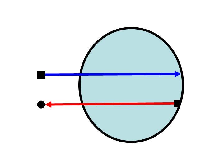 Notice the relationship between these arrows and the wall of the circle. The arrow origin or head may be located at the perimeter of the circle, or outside of the circle. If we replace the arrows for tracks and the circle for the brain (the perimeter the cerebral cortex) we will understand the tracts called "Projection Fibers." They carry information in and out of the brain. Some examples of "Projection Fibers" are: Visual Pathways, and the Cortico-spinal or pyramidal tract.
Projection Fibers Types
- Efferent (Going away)
- Cortico-spinal tract (Pyramidal tract)
- Cortico-nuclear system
- Fronto-pontine tract
- Afferent (Coming towards)
- Spino-thalamo-cortical tract
- Visual pathway
- Auditory pathway
- Medial Lemniscus system
Associative Fibers
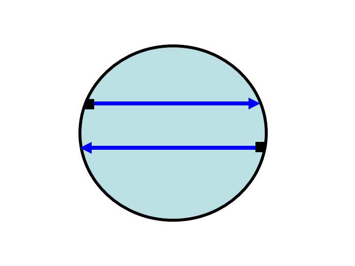
In this other example the arrows have both origin and end point within the circle "connecting" different points of the perimeter. Using the same model, this represents fibers that connect different areas of the cerebral cortex, within the same hemisphere or between them. These types of fibers are called "Associative Fibers." They carry information between similar areas of processing, or from lower to higher levels of cortical complexity. Two examples of these fibers are the Corpus Callosum and the arcuate fasciculus.
Association Fibers Types
- Intrahemispheric
- Superior Longitudinal Fasciculus
- Inferior Longitudinal Fasciculus
- Superior Occipito-Frontal Fasciculus
- Cingulum
- Fornix
- Interhemispheric
- Body of Corpus Callosum
- Forceps Major of Corpus Callosum
- Forceps Minor of Corpus Callosum
- Anterior Commisure
- Posterior Commisure
Integrative Fibers
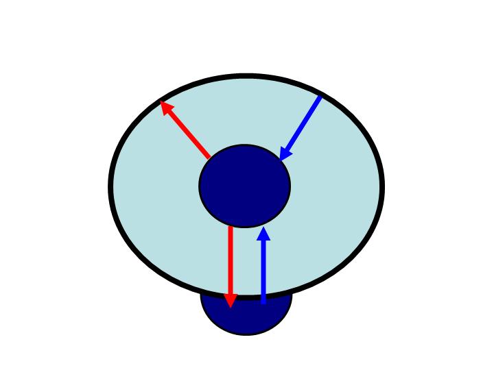 In this model we have arrows that have either the origin or end point within the circle but one of the ends is not located in the perimeter of the circle.
This represents fibers connecting the cerebral cortex with other gray matter areas of the CNS (e.g.: the thalamus, the cerebellum). Fibers connecting cerebral non-cortical gray matter areas are also considered within this group. These are the "Integrative Fibers." Two examples of fibers of this type are the thalamic-frontal fibers and the rubro-thalamic fibers.
Integrative Fibers Types
- Thalamo-frontal fibers
- Fronto-thalamic fibers
- Fronto-striatal fibers
- Thalamo-lenticular fibers
- Rubro thalamic fibers
- Mamilo-thalamic fibers
- Ponto-rubro-thalamic fibers
- Fronto-ponto-cerebellar fibers
- Nigro-thalamo-frontal fibers
- Medial Longitudinal Fascicle
- Many others
Tracts on DTI
DTI stands for Diffusion Tensor Imaging. This is an imaging technique based on the 3D shape of water diffusion. Free diffusion occurs equally in all directions. This is termed "isotropic" diffusion. If the water diffuses in a milieu having barriers, the diffusion will be uneven. In such a case, the relative-mobility of the molecules from the origin has a shape different from a sphere, most frequently an ellipsoid. Barriers can be many things --cell membranes, axons, myelin, etc; but in white matter the principal barrier is the myelin sheath of axons. Bundles of axons provide a barrier to perpendicular diffusion and a path for parallel diffusion along the orientation of the fibers. This is termed "anisotropic" diffusion.
Anisotropic diffusion is expected to be increased in areas of high mature axonal order. Conditions where the myelin or the structure of the axon are disrupted, such as trauma, tumors, and inflammation reduce anisotropy, as the barriers are affected by destruction or disorganization.
Anisotropy is measured in several ways. One way is by a ratio called "fractional anisotropy" (FA). An anisotropy of "0" corresponds to a perfect sphere, whereas 1 is an ideal linear diffusion. Well defined tracts have FA larger than 0.20. Few regions have FA larger than 0.90. The number gives us information of how asymmetric the diffusion is but says nothing of the direction.
Each anisotropy is linked to a orientation of the predominant axis (predominant direction of the diffusion). Post-processing programs are able to extract this directional information.
This additional information is difficult to represent on 2D grey-scaled images. To overcome this problem a color code is introduced . Basic colors can tell the observer how the fibers are oriented in a 3D-coordinate system: This is termed an "anisotropic map." Our software encodes the colors in this way:
- Red indicates directions in the X axis: right to left or left to right.
- Green indicates directions in the Y axis: posterior to anterior or from anterior to posterior.
- Blue indicates directions in the Z axis: foot-to-head direction or vice versa.
Notice that the technique is unable to discriminate the "positive" or "negative" direction in the same axis.
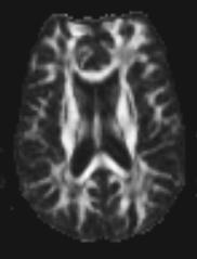 Fractional anisotropy image. White pixels (dots) correspond to high values of fractional anisotropy (FA). Dark pixels correspond to low values of FA. White matter consists of axons, which serve as barriers for free water diffusion, and explains the high anisotropy which is bright compared to cortex where there is less structure and more free diffuse resulting in lower sign.
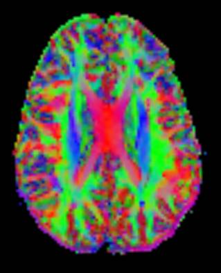 Color coded fractional anisotropy map. Pixels are now displayed in colors to reveal the predominant direction of the diffusion tensor. Green shows fibers oriented anterior-to-posterior or posterior-to-anterior. Red shows fibers oriented right-to-left or left-to-right (e.g.: corpus callosum). Blue shows fibers oriented head-to-foot or vice versa (e.g.: the pyramidal tracts in the corona radiata, lateral to the corpus callosum).
Main Cerebral Tracts on
Orthogonal Fractional Anisotropy Maps
Cerebral tracts may be presented in 2D color images in: axial, coronal, and sagittal planes. The relational topographic appearance of the tracts are better identified in planes that are perpendicular to the major axis of the tract. For example, the corpus callosum which is an axial structure is better defined in the sagittal or coronal view. Thus, tracts going anterior-posterior or posterior-anterior are better seen in coronal view. Descending and ascending tracts are better depicted in axial view (Figure 1).
Figure 1. Axial FA Map. We have targeted blue fibers which encodes for foot-head or head-foot direction.
- Ext: External.
- IC: Internal Capsule
- IOFF: Inferior Occipito-Frontal Fasciculus
- Post: Posterior
- Cort: Cortical
- Thal: Thalamic
- Bulb: Bulbar
- ILF: Inferior Longitudinal Fasciculus
Notice that the portion of the ILF and IOFF shown are just some bundles ascending in the posterior portions as these fasciculi are predominantly posterio-anterior oriented.
Coronal view (figure 2) is better to show the fibers oriented posteior-anterior or anterior-posterior, coded in green.
Figure 2. Coronal FA Map.
- SOFF: Superior Occipito-frontal Fasciculus
- SLF: Superior Longitudinal Fasciculus
- IOFF: Inferior Occipito-frontal fasciculus
- ILF: Inferior Longitudinal Fasciculus.
- SCP: Superior Cerebellar Peduncle
The sagittal plane (figure 3) best provides information on interhemispherical fibers going right to left or viceversa (red) or anterior-posterior (green). These are the corpus callosum and the anterior commissure.
Figure 3. Saggital FA Map. Interhemispheric fibers are red in the midsagittal cut. Horizontal portion of the cingulum above the corpus callosum appears green. The green bundle in the inferior left corresponds to the medial part of the superior cerebellar peduncle.
Subcortical U fibers appear various colors due to multiple intersecting planes.